corrplot包与ggcorrplot相关图（一）

会员服务 ·

corrplot包与ggcorrplot相关图（一）

2019 年 4 月 10 日 R语言中文社区

作者：李誉辉

四川大学在读研究生

简介：
相关图是基于相关系数矩阵绘制的图。
通常是将1个变量映射到多个视觉元素，所以看起来很花哨。
如果是椭圆：

则椭圆的色相对应相关性的正负，
颜色深浅对应相关性绝对值大小，越深则绝对值越大。
椭圆的形状对应相关性绝对值大小，默认越扁，则相关性绝对值越大。

如果是圆，则圆的面积对应相关性大小，
如果是扇形，则扇形的弧度对应相关性大小。

相关系数：
自变量X和因变量Y的协方差/标准差的乘积。也可以反映两个变量变化时是同向还是反向，
如果同向变化就为正，反向变化就为负。
它消除了两个变量变化幅度的影响，而只是单纯反应两个变量每单位变化时的相似程度。

表达式：
cor(x, y = NULL, use = "everything", method = c("pearson", "kendall", "spearman"))

参数解释：

x 为数字型向量，矩阵或数据框，表示自变量
y 表示应变量，默认y=x

2个向量计算得到一个值，n个变量组成的数据框计算得到长度为n*n维度的矩阵。
绘制相关图主要涉及2个包：corrplot, ggcorrplot，后一个是ggplot2的扩展包。

计算相关系数矩阵：

 1height <- c(6, 5.92, 5.58, 5.83)
 2wei <- c(20, 15, 7, 12)
 3cor(height, exp(height))
 4cor(height, wei)
 5ncol(mtcars)
 6dim(cor(mtcars)) # 
 7class(cor(mtcars))
 8colnames(cor(mtcars))
 9row.names(cor(mtcars))
10
11# 展示系数矩阵,保留3位小数，
12DT::datatable(round(cor(mtcars), 3), 
13              options = list(pageLength = 11)) # 显示11行

1## [1] 0.9983074
2## [1] 0.9628811
3## [1] 11
4## [1] 11 11
5## [1] "matrix"
6##  [1] "mpg"  "cyl"  "disp" "hp"   "drat" "wt"   "qsec" "vs"   "am"   "gear"
7## [11] "carb"
8##  [1] "mpg"  "cyl"  "disp" "hp"   "drat" "wt"   "qsec" "vs"   "am"   "gear"
9## [11] "carb"

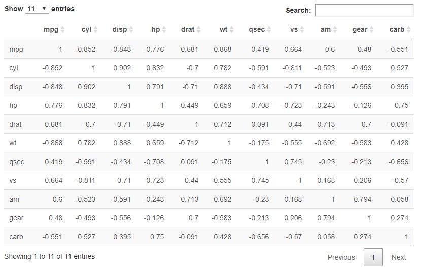
（原图可交互）

corrplot包绘图：

结果按行和按列排是一样的，说明，只要cor(x,y)中，只要x=y，按行排和按列排没有区别。

1library(corrplot)
2corrplot(cor(mtcars))

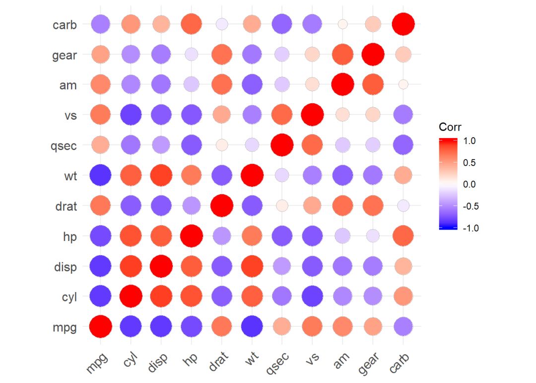
1library(ggplot2)
2library(ggcorrplot)
3
4ggcorrplot(cor(mtcars), method="circle")

1.corrplot包

1.1

语法与参数

语法：

 1corrplot(corr,
 2    method = c("circle", "square", "ellipse", "number", "shade", "color", "pie"),
 3    type = c("full", "lower", "upper"), add = FALSE,
 4    col = NULL, bg = "white", title = "",  is.corr = TRUE,      
 5    diag = TRUE, outline = FALSE, mar = c(0,0,0,0),
 6    addgrid.col = NULL, addCoef.col = NULL, addCoefasPercent = FALSE, 
 7    order = c("original", "AOE", "FPC", "hclust", "alphabet"),
 8    hclust.method = c("complete", "ward", "single", "average",
 9                      "mcquitty", "median", "centroid"),
10    addrect = NULL, rect.col = "black", rect.lwd = 2,
11    tl.pos = NULL, tl.cex = 1,
12    tl.col = "red", tl.offset = 0.4, tl.srt = 90,
13    cl.pos = NULL, cl.lim = NULL,
14    cl.length = NULL, cl.cex = 0.8, cl.ratio = 0.15, 
15    cl.align.text = "c",cl.offset = 0.5,
16    addshade = c("negative", "positive", "all"),
17    shade.lwd = 1, shade.col = "white",
18    p.mat = NULL, sig.level = 0.05,
19    insig = c("pch","p-value","blank", "n"),
20    pch = 4, pch.col = "black", pch.cex = 3,
21    plotCI = c("n","square", "circle", "rect"),
22    lowCI.mat = NULL, uppCI.mat = NULL, ...)

关键参数：

corr, 需要可视化的相关系数矩阵，
method, 指定可视化的形状，可以是circle圆形(默认)，square方形，
ellipse, 椭圆形，number数值，shade阴影，color颜色，pie饼图。
type，指定显示范围，可以是full完全(默认)，lower下三角，upper上三角。
col, 指定图形展示的颜色，默认以均匀的颜色展示。
支持grDevices包中的调色板，也支持RColorBrewer包中调色板。
bg, 指定背景颜色。
add, 表示是否添加到已经存在的plot中。默认FALSE生成新plot。
title, 指定标题，
is.corr，是否为相关系数绘图，默认为TRUE,FALSE则可将其它数字矩阵进行可视化。
diag, 是否展示对角线上的结果，默认为TRUE，
outline, 是否添加圆形、方形或椭圆形的外边框，默认为FALSE。
mar，设置图形的四边间距。数字分别对应(bottom, left, top, right)。
addgrid.col, 设置网格线颜色，当指定method参数为color或shade时，默认的网格线颜色为白色，其它method则默认为灰色，也可以自定义颜色。
addCoef.col，设置相关系数值的颜色，只有当method不是number时才有效。
addCoefasPercent, 是否将相关系数转化为百分比形式，以节省空间，默认为FALSE。
order, 指定相关系数排序的方法, 可以是original原始顺序，AOE特征向量角序，
FPC第一主成分顺序，hclust层次聚类顺序，alphabet字母顺序。
hclust.method, 指定hclust中细分的方法，只有当指定order参数为hclust时有效，
有7种可选：complete, ward, single, average, mcquitty, median, centroid。
addrect，是否添加矩形框，只有当指定order参数为hclust时有效，默认不添加，用整数指定即可添加。
rect.col, 指定矩形框的颜色。
rect.lwd, 指定矩形框的线宽。
tl.pos, 指定文本标签(变量名称)相对绘图区域的位置，为"lt"(左侧和顶部),
"ld"(左侧和对角线), "td"(顶部和对角线),"d"(对角线),"n"(无)之一。
当type="full"时,默认"lt"。
当type="lower"时，默认"ld"。
当type="upper"时，默认"td"。
tl.cex, 设置文本标签的大小。
tl.col, 设置文本标签的颜色。
cl.pos, 设置图例位置，为"r"(右边), "b"(底部),"n"(无)之一。
当type="full"/"upper"时，默认"r"; 当type="lower"时，默认"b"。
addshade, 表示给增加阴影，只有当method="shade"时有效。
为"negative"(对负相关系数增加阴影),负相关系数的阴影是135度；
"positive"(对正相关系数增加阴影), 正相关系数的阴影是45度；
"all"(对所有相关系数增加阴影)，之一。
shade.lwd, 指定阴影线宽。
shade.col, 指定阴影线的颜色。

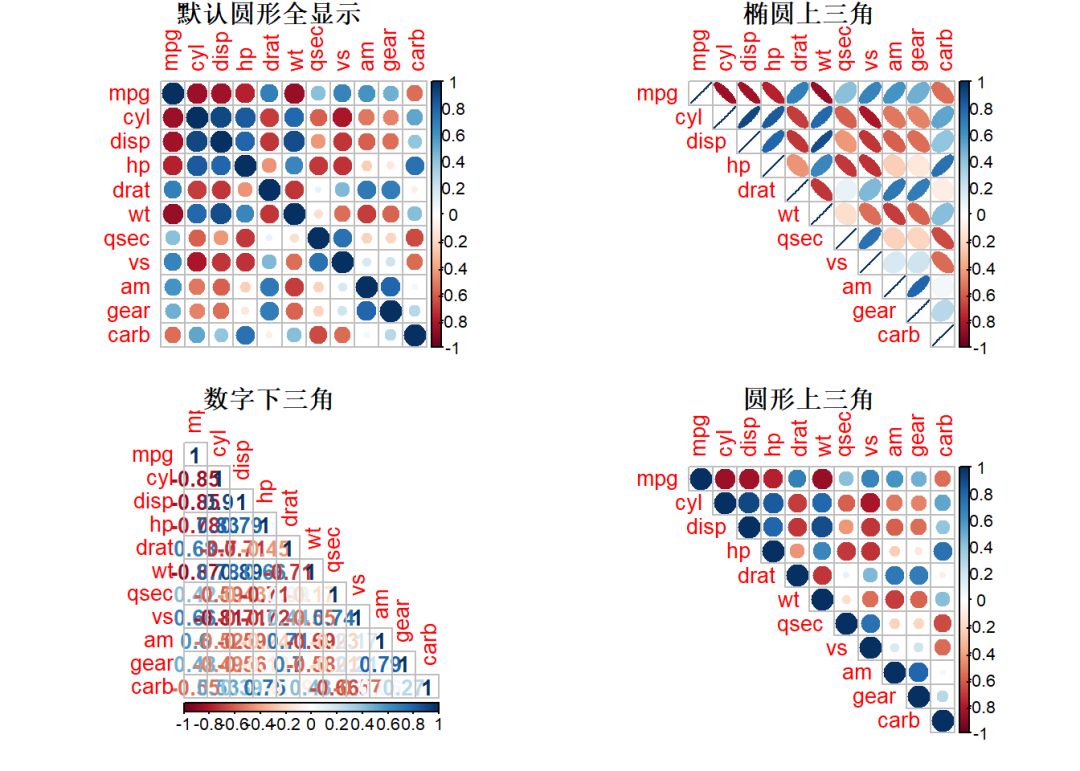
1.2

method与type

 1library(corrplot)
 2library(showtext)
 3mat_cor <- cor(mtcars)
 4
 5par(mfrow = c(2,2)) # 多图排版，2x2矩阵排列
 6
 7corrplot(mat_cor, title = "默认圆形全显示", # 默认method为圆形，默认type为full
 8         mar = c(1,1,1,1)) # 指定边距，否则标题显示不完全
 9corrplot(mat_cor, method = "ellipse", type = "upper", title = "椭圆上三角",
10         mar = c(1,1,1,1))
11corrplot(mat_cor, method = "number", type = "lower", title = "数字下三角",
12         mar = c(1,1,1,1))
13corrplot(mat_cor, method = "circle", type = "upper", title = "圆形上三角",
14         mar = c(1,1,1,1))
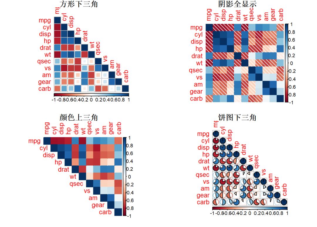
15corrplot(mat_cor, method = "square", type = "lower", title = "方形下三角",
16         mar = c(1,1,1,1))
17corrplot(mat_cor, method = "shade", type = "full", title = "阴影全显示",
18         mar = c(1,1,1,1))
19corrplot(mat_cor, method = "color", type = "upper", title = "颜色上三角",
20         mar = c(1,1,1,1))
21corrplot(mat_cor, method = "pie", type = "lower", title = "饼图下三角",
22         mar = c(1,1,1,1))

1.3

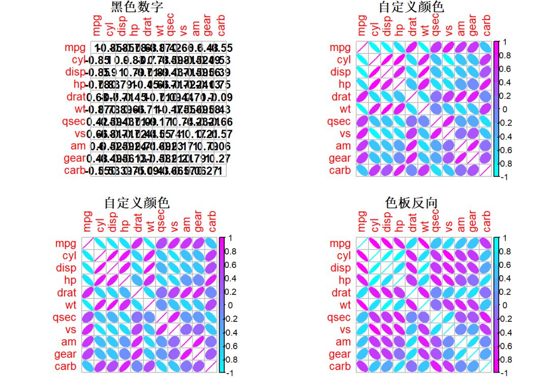
col颜色

颜色可以自定义，支持grDevices包中的调色板。也支持RColorBrewer中的调色板。

 1# 自定义色板
 2color_1 <- colorRampPalette(c("cyan", "magenta"))
 3color_2 <- colorRampPalette(c("magenta", "cyan")) # 色板反向
 4palette_1 <- RColorBrewer::brewer.pal(n=11, name = "RdYlGn")
 5palette_2 <- rev(palette_1) # 色板反向
 6
 7par(mfrow = c(2, 2))
 8
 9corrplot(mat_cor, method = "number", col = "black", cl.pos = "n", 
10         title = "黑色数字", mar = c(1,1,1,1))
11
12corrplot(mat_cor, method = "ellipse", col = color_1(10), 
13         title = "自定义颜色", mar = c(1,1,1,1))
14
15corrplot(mat_cor, method = "ellipse", col = color_1(200), # 矩阵维度不够大，所以颜色没区别
16         title = "自定义颜色", mar = c(1,1,1,1))
17
18corrplot(mat_cor, method = "ellipse", col = color_2(10), 
19         title = "色板反向", mar = c(1,1,1,1))
20
21par(mfrow = c(1,1))
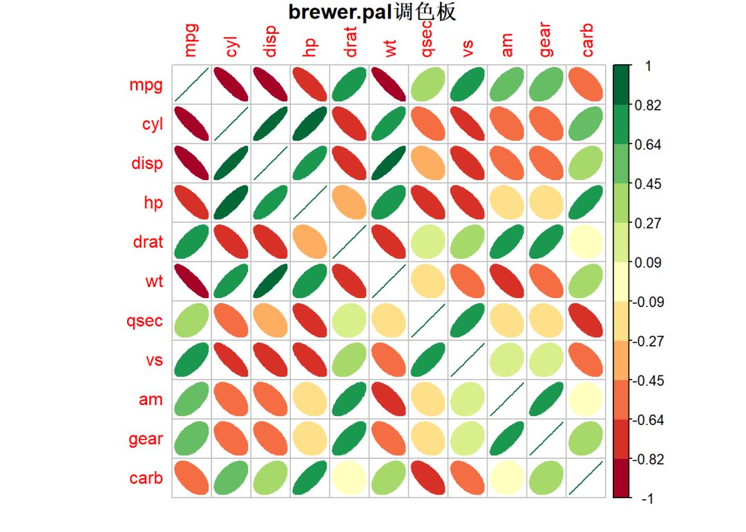
22corrplot(mat_cor, method = "ellipse", col = palette_1,
23         title = "brewer.pal调色板", mar = c(1,1,1,1))
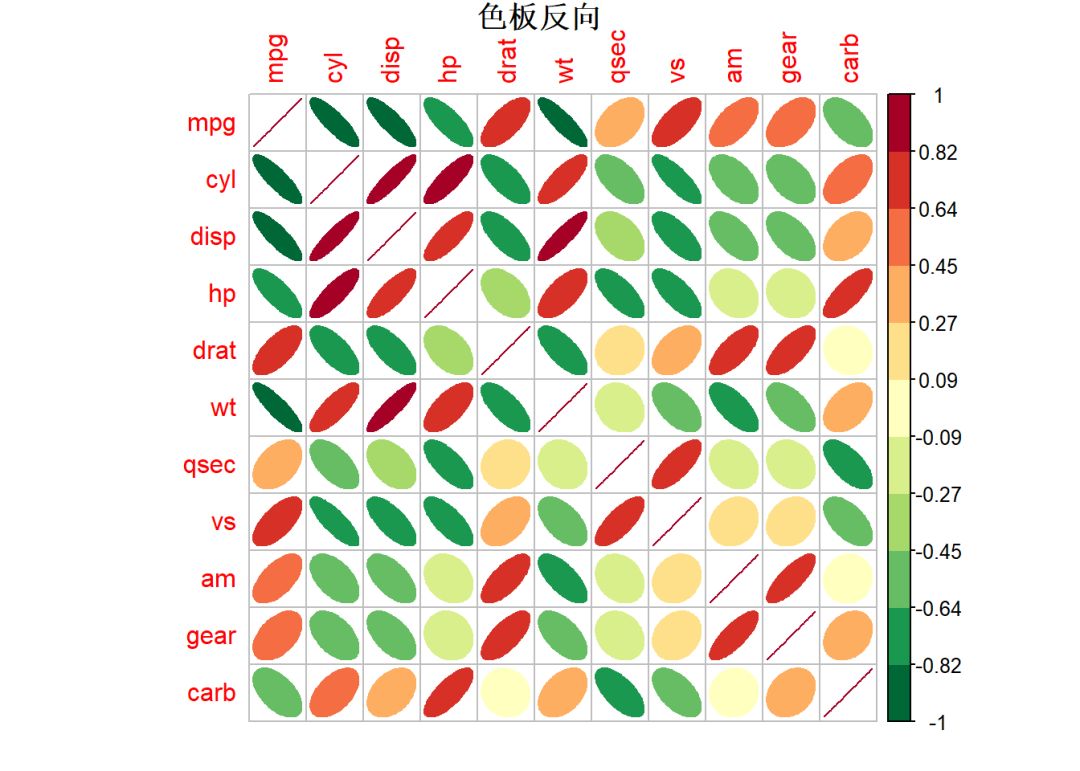
24corrplot(mat_cor, method = "ellipse", col = palette_2,
25         title = "色板反向", mar = c(1,1,1,1))  
26

1.4

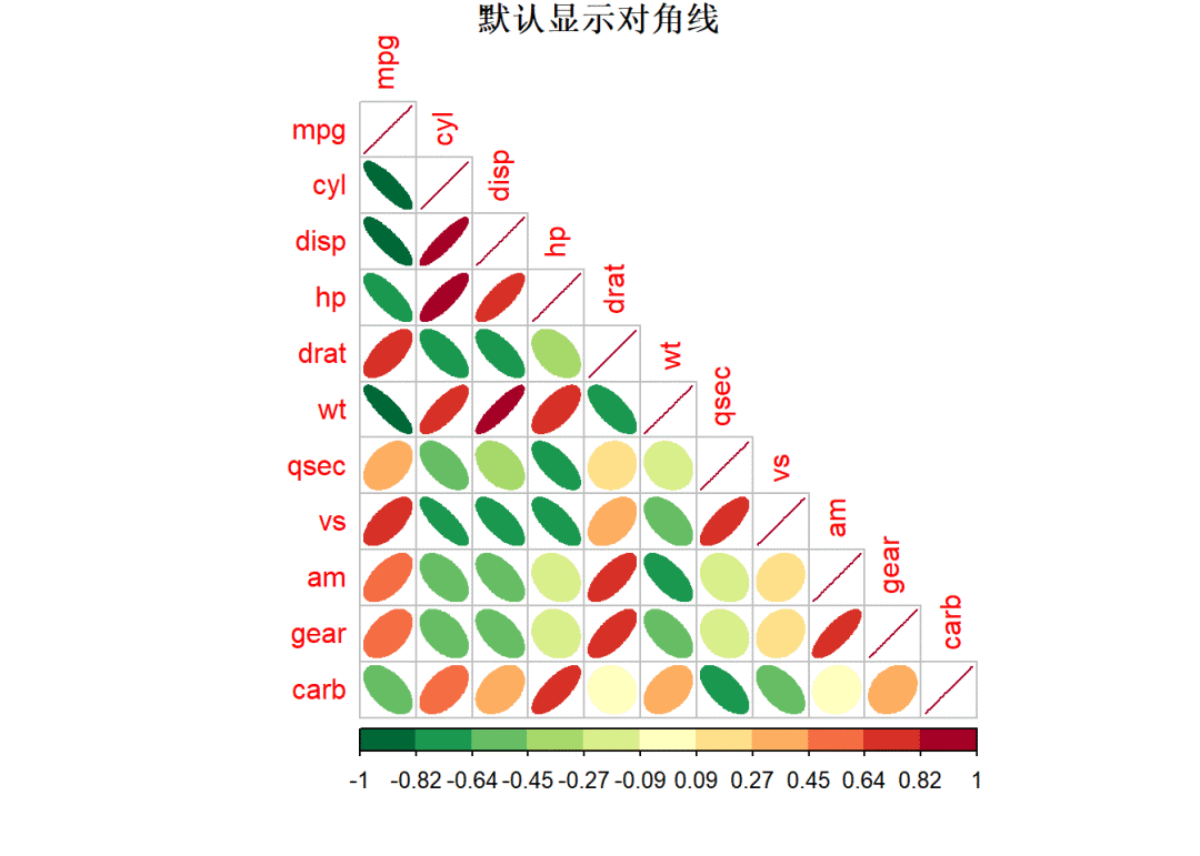
diag和bg

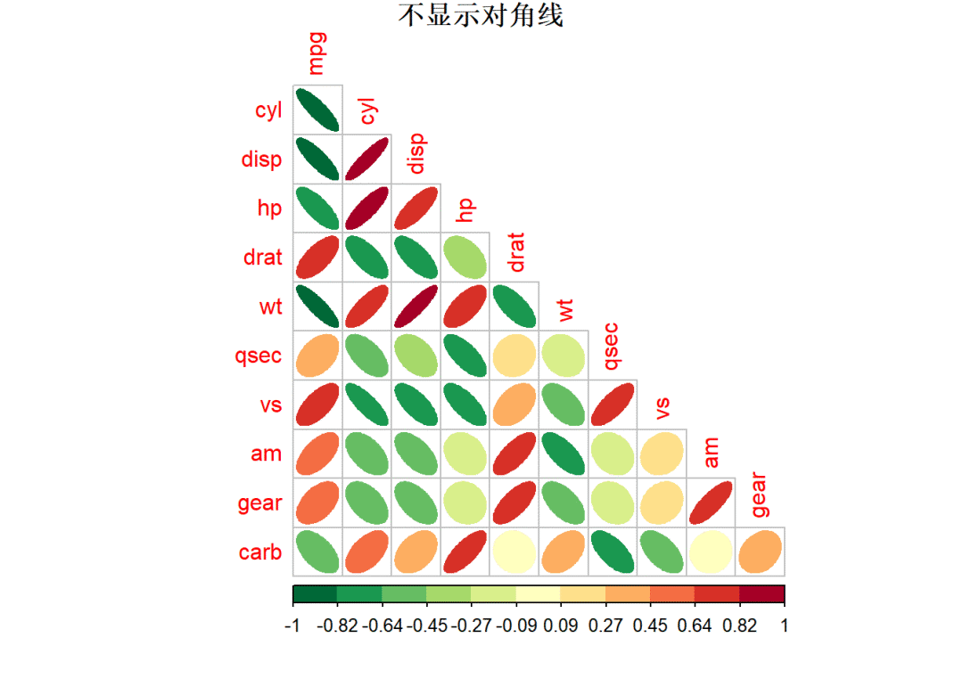
1corrplot(mat_cor, method = "ellipse", type = "lower", col = palette_2,
2         title = "默认显示对角线",diag = TRUE, mar = c(1,1,1,1))
3corrplot(mat_cor, method = "ellipse", type = "lower", col = palette_2,
4         title = "不显示对角线", diag = FALSE, mar = c(1,1,1,1))
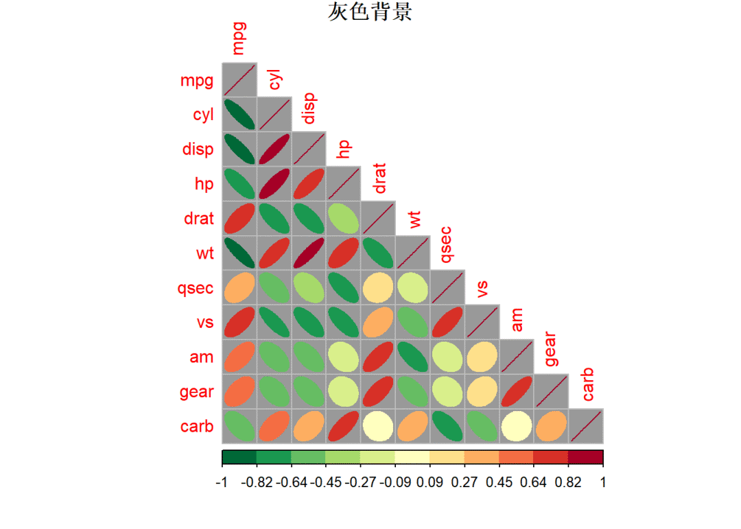
5corrplot(mat_cor, method = "ellipse", type = "lower", col = palette_2,
6         title = "灰色背景", bg = "gray60", mar = c(1,1,1,1))
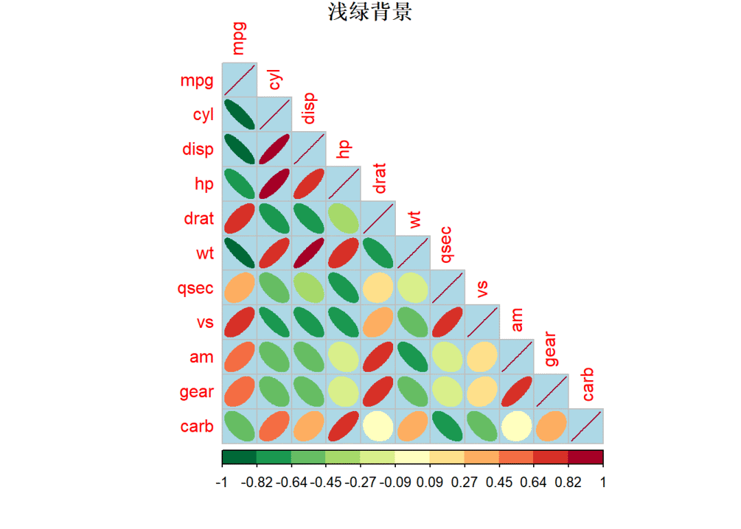
7corrplot(mat_cor, method = "ellipse", type = "lower", col = palette_2,
8         title = "浅绿背景", bg = "lightblue", mar = c(1,1,1,1))

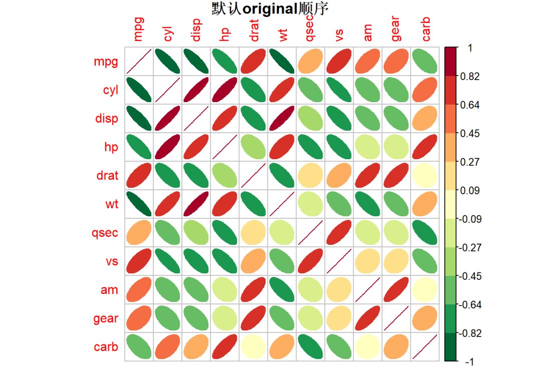
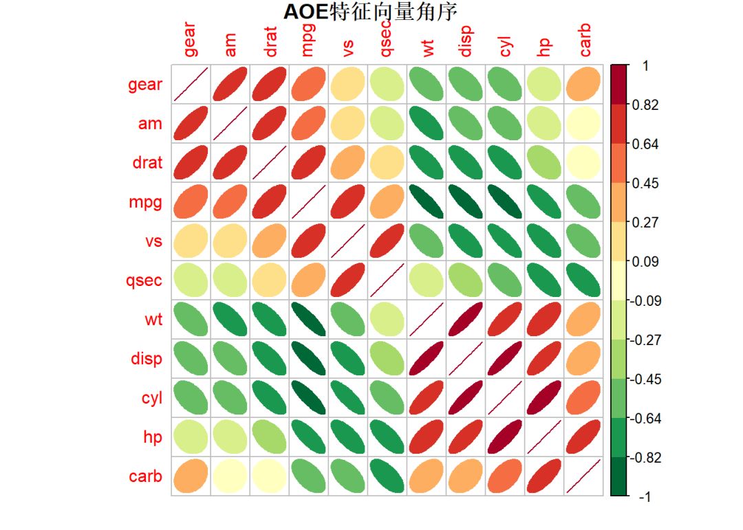
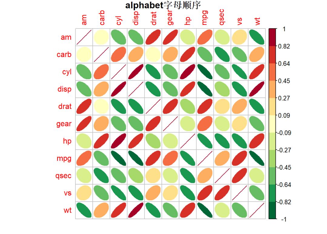
1.5

order顺序

 1corrplot(mat_cor, method = "ellipse", col = palette_2,
 2         title = "默认original顺序", diag = TRUE, mar = c(1,1,1,1))
 3corrplot(mat_cor, method = "ellipse", order = "AOE",  col = palette_2,
 4         title = "AOE特征向量角序", diag = TRUE, mar = c(1,1,1,1))
 5corrplot(mat_cor, method = "ellipse", order = "FPC",  col = palette_2,
 6         title = "FPC第一主成分顺序", diag = TRUE, mar = c(1,1,1,1))
 7corrplot(mat_cor, method = "ellipse", order = "hclust",  col = palette_2,
 8         title = "hclust层次聚类顺序", diag = TRUE, mar = c(1,1,1,1))
 9corrplot(mat_cor, method = "ellipse", order = "alphabet",  col = palette_2,
10         title = "alphabet字母顺序", diag = TRUE, mar = c(1,1,1,1))

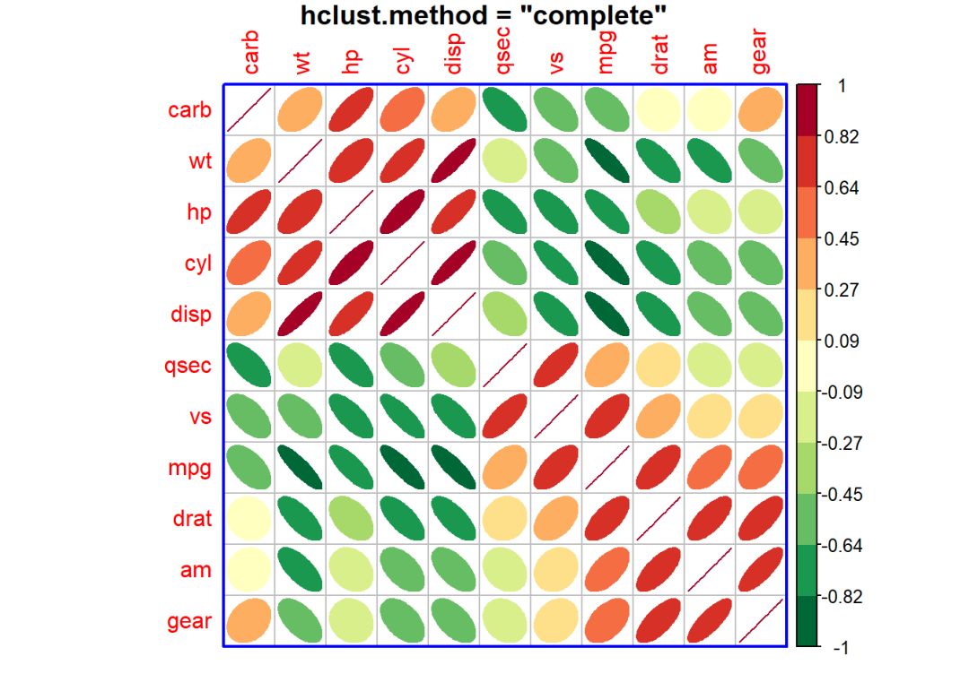
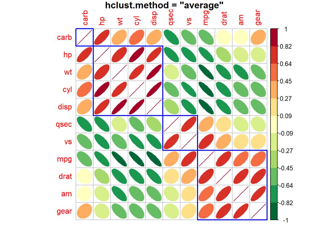
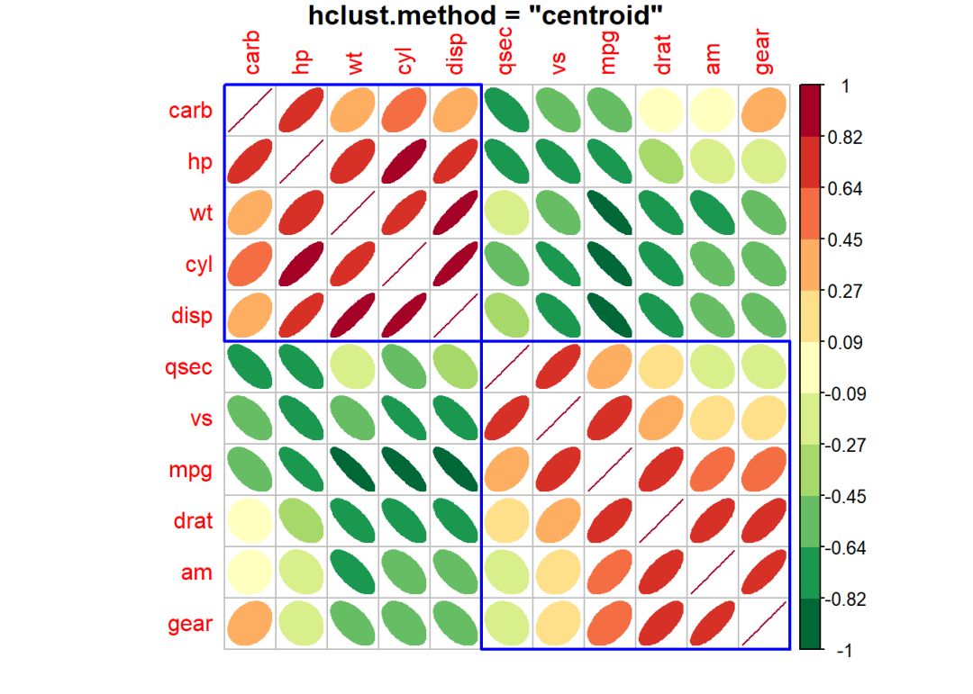
1.6

hclust.method和addrect

只有当order="hclust"才有效。

 1corrplot(mat_cor, method = "ellipse", order = "hclust",  col = palette_2,
 2         hclust.method = "complete", addrect = 1, rect.col = "blue", rect.lwd = 2,
 3         title = "hclust.method = \"complete\"", diag = TRUE, mar = c(1,1,1,1))
 4corrplot(mat_cor, method = "ellipse", order = "hclust",  col = palette_2,
 5         hclust.method = "ward", addrect = 2, rect.col = "blue", rect.lwd = 2,
 6         title = "hclust.method = \"ward\"", diag = TRUE, mar = c(1,1,1,1))
 7corrplot(mat_cor, method = "ellipse", order = "hclust",  col = palette_2,
 8         hclust.method = "single", addrect = 3, rect.col = "blue", rect.lwd = 2,
 9         title = "hclust.method = \"single\"", diag = TRUE, mar = c(1,1,1,1))
10corrplot(mat_cor, method = "ellipse", order = "hclust",  col = palette_2,
11         hclust.method = "average", addrect = 4, rect.col = "blue", rect.lwd = 2,
12         title = "hclust.method = \"average\"", diag = TRUE, mar = c(1,1,1,1))
13corrplot(mat_cor, method = "ellipse", order = "hclust",  col = palette_2,
14         hclust.method = "mcquitty", addrect = 2, rect.col = "blue", rect.lwd = 2,
15         title = "hclust.method = \"mcquitty\"", diag = TRUE, mar = c(1,1,1,1))
16corrplot(mat_cor, method = "ellipse", order = "hclust",  col = palette_2,
17         hclust.method = "median", addrect = 2, rect.col = "blue", rect.lwd = 2,
18         title = "hclust.method = \"median\"", diag = TRUE, mar = c(1,1,1,1))
19corrplot(mat_cor, method = "ellipse", order = "hclust",  col = palette_2,
20         hclust.method = "centroid", addrect = 2, rect.col = "blue", rect.lwd = 2,
21         title = "hclust.method = \"centroid\"", diag = TRUE, mar = c(1,1,1,1))

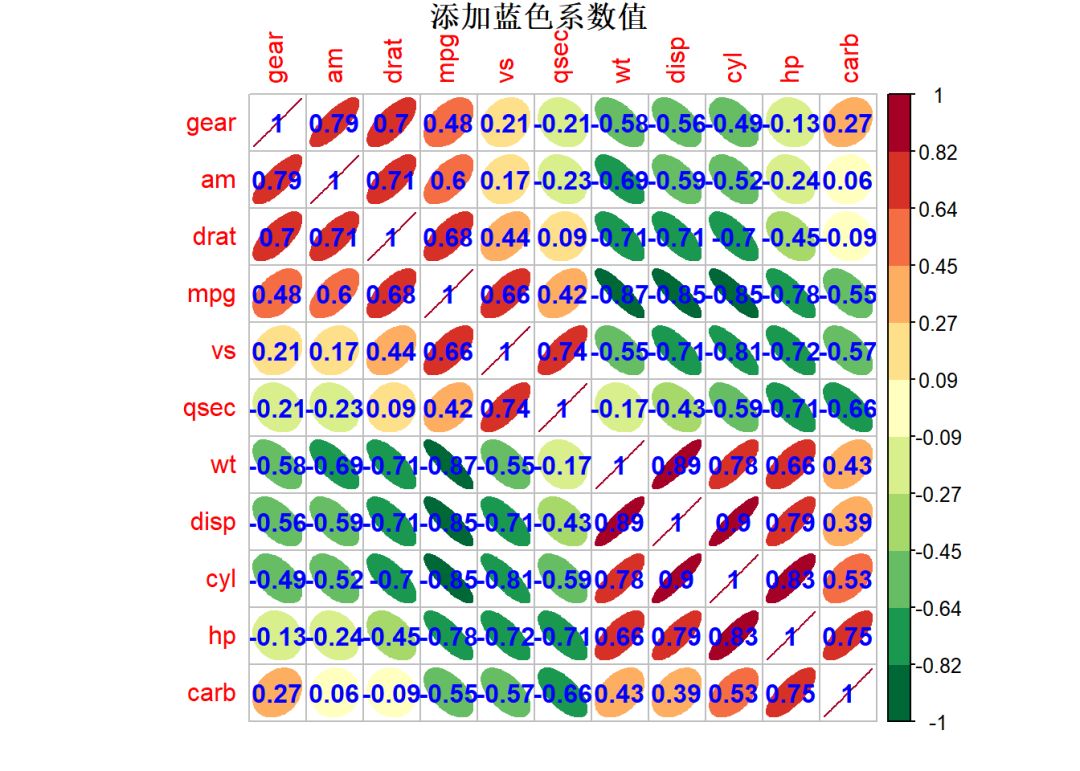
1.7

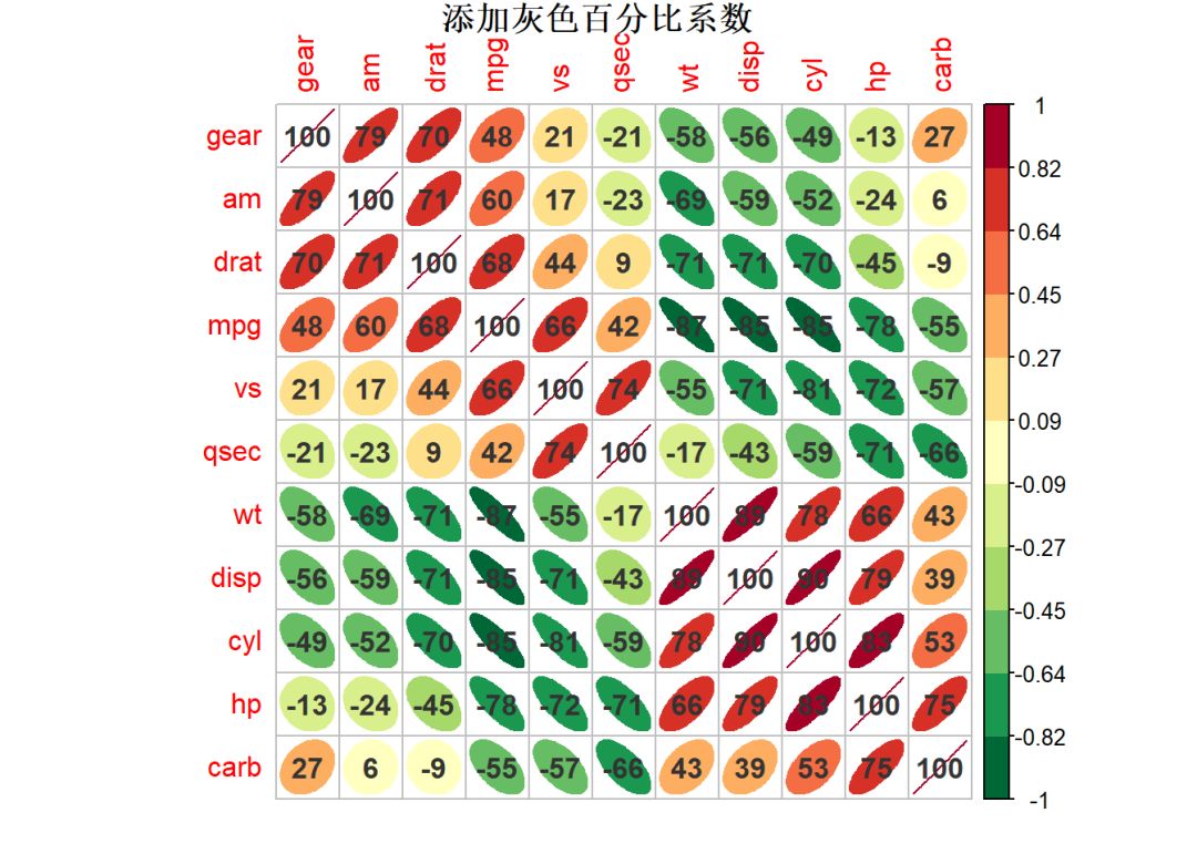
addCoef.col与addCoefasPercent

 1corrplot(mat_cor, method = "ellipse", order = "AOE",  col = palette_2, 
 2         addCoef.col = "blue",
 3         title = "添加蓝色系数值", diag = TRUE, mar = c(1,1,1,1))
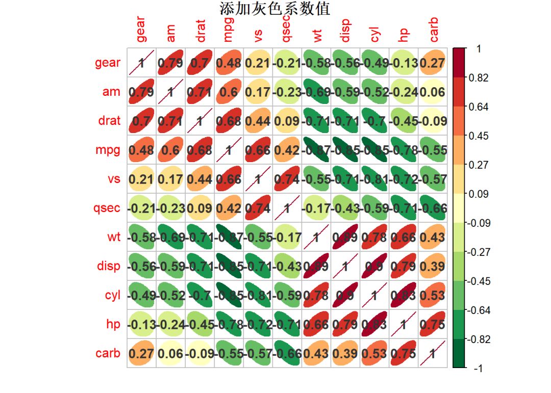
 4corrplot(mat_cor, method = "ellipse", order = "AOE",  col = palette_2, 
 5         addCoef.col = "gray20",
 6         title = "添加灰色系数值", diag = TRUE, mar = c(1,1,1,1))
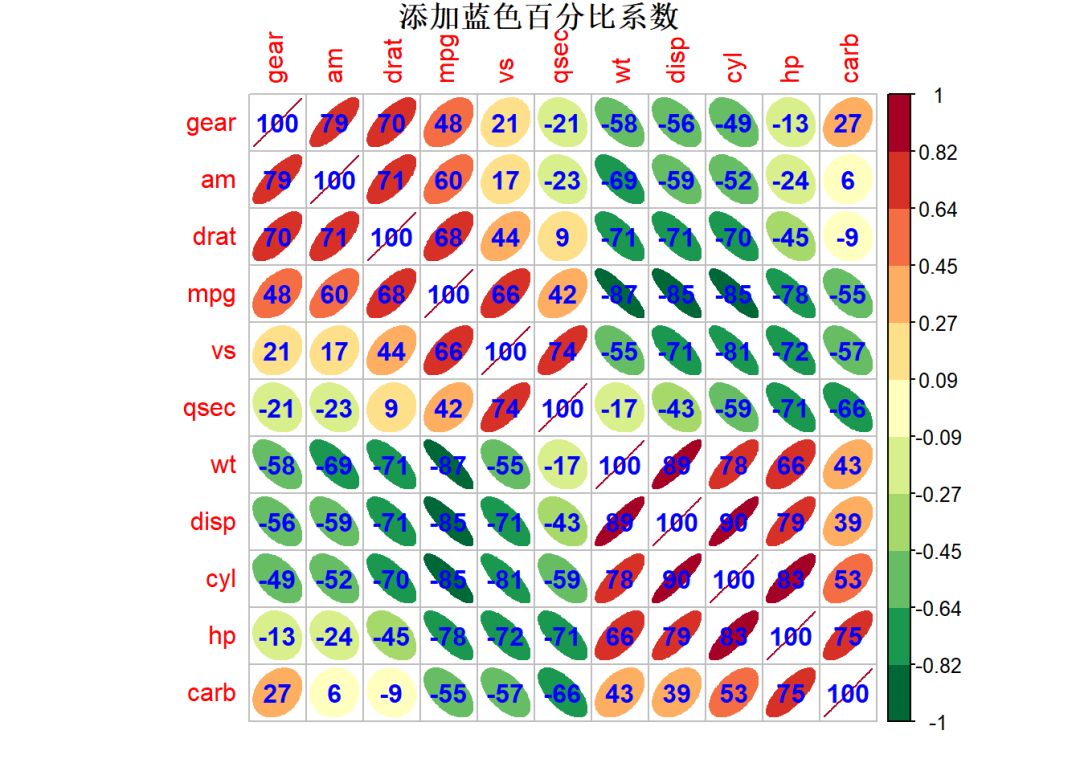
 7
 8corrplot(mat_cor, method = "ellipse", order = "AOE",  col = palette_2, 
 9         addCoef.col = "blue", addCoefasPercent = TRUE,
10         title = "添加蓝色百分比系数", diag = TRUE, mar = c(1,1,1,1))
11corrplot(mat_cor, method = "ellipse", order = "AOE",  col = palette_2, 
12         addCoef.col = "gray20", addCoefasPercent = TRUE,
13         title = "添加灰色百分比系数", diag = TRUE, mar = c(1,1,1,1))

——————————————

往期精彩：

登录查看更多

相关内容