如何构建一个生产环境的推荐系统

2020 年 9 月 20 日 DataFunTalk

文章作者：哥不是小萝莉，来源：

https://www.cnblogs.com/smartloli/

导读： 现在互联网上的内容很多，我们可能每天都会接受来自不同消息。例如，电商网站、阅读博客、各类新闻文章等。但是，这些消息并不是所有的内容你都感兴趣，可能你只对技术博客感兴趣，或者某些新闻感兴趣等等。而这些内容如何去满足用户的需求呢？我们需要一个精准的解决方案来简化用户的发现过程。

01 推荐系统的作用是啥？

简而言之，推荐系统就是一个发现用户喜好的系统。系统从数据中学习并向用户提供有效的建议。如果用户没有特意搜索某项物品，则系统会自动将该项带出。这样看起很神奇，比如，你在电商网站上浏览过某个品牌的鞋子，当你在用一些社交软件、短视频软件、视频软件时，你会惊奇的发现在你所使用的这些软件中，会给你推荐你刚刚在电商网站上浏览的过的鞋子。

其实，这得益于推荐系统的过滤功能。我们来看看一张简图，如下图所示：

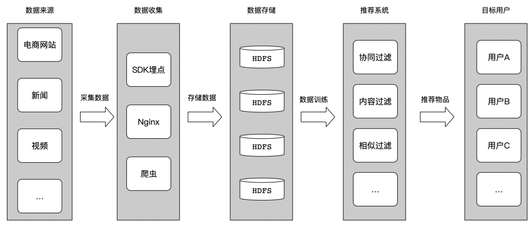
从上图中，我们可以简单的总结出，整个数据流程如下：

数据来源：负责提供数据来源，比如用户在电商网站、新闻、视频等上的用户行为，作为推荐训练的数据来源；
数据采集：用户产生了数据，我们需要将这些数据进行收集，比如SDK埋点采集、Nginx上报、爬虫等方式来获取数据；
数据存储：获取这些数据后，需要对这些数据进行分类存储、清洗等，比如大数据里面用的最多的HDFS，或者构建数据仓库Hive表等；
推荐系统：数据分类、清洗后好，有了推荐系统需要的数据，然后使用推荐系统中的各种模型、比如协同过滤、内容过滤、相似过滤、用户矩阵等，来训练这些用户数据，得到训练结果；
目标用户：通过推荐系统，对用户数据进行训练后，得出训练结果，将这些结果，推荐给目标用户。

02 依赖准备

我们使用Python来够构建推荐系统模型，需要依赖如下的Python依赖包：

pip install numpypip install scipypip install pandaspip install jupyterpip install requests

这里为简化Python的依赖环境，推荐使用Anaconda3。这里面集成了很多Python的依赖库，不用我们在额外去关注Python的环境准备。

接着，我们加载数据源，代码如下：

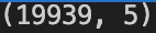
import pandas as pdimport numpy as np
df = pd.read_csv('resource/events.csv')df.shapeprint(df.head())

结果如下：

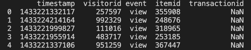
使用df.head()会打印数据前5行数据：

timestamp：时间戳
visitorid：用户ID
event：事件类型
itemid：物品ID
transactionid：事务ID

使用如下代码，查看事件类型有哪些：

print(df.event.unique())

结果如下：

从上图可知，类型有三种，分别是：view、addtocart、transaction。

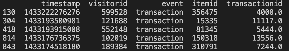
为了简化起见，以transaction类型为例子。代码如下所示：

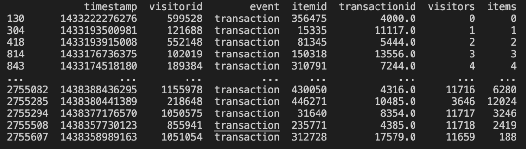
trans = df[df['event'] == 'transaction']trans.shapeprint(trans.head())

结果如下图所示：

接着，我们来看看用户和物品的相关数据，代码如下：

visitors = trans['visitorid'].unique()items = trans['itemid'].unique()print(visitors.shape)print(items.shape)

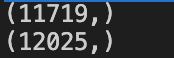
我们可以获得11719个去重用户和12025个去重物品。

构建一个简单而有效的推荐系统的经验法则是在不损失精准度的情况下减少数据的样本。这意味着，你只能为每个用户获取大约50个最新的事务样本，并且我们仍然可以得到期望中的结果。

代码如下所示：

trans2 = trans.groupby(['visitorid']).head(50)print(trans2.shape)

真实场景中，用户ID和物品ID是一个海量数字，人为很难记住，比如如下代码：

trans2['visitors'] = trans2['visitorid'].apply(lambda x : np.argwhere(visitors == x)[0][0])trans2['items'] = trans2['itemid'].apply(lambda x : np.argwhere(items == x)[0][0])
print(trans2)

结果如下图所示：

03 构建矩阵

1. 构建用户-物品矩阵

从上面的代码执行的结果来看，目前样本数据中有11719个去重用户和12025个去重物品，因此，我们接下来构建一个稀疏矩阵。需要用到如下Python依赖：

from scipy.sparse import csr_matrix

实现代码如下所示：

occurences = csr_matrix((visitors.shape[0], items.shape[0]), dtype='int8')def set_occurences(visitor, item):    occurences[visitor, item] += 1trans2.apply(lambda row: set_occurences(row['visitors'], row['items']), axis=1)print(occurences)

结果如下所示：

(0, 0)        1  (1, 1)        1  (1, 37)       1  (1, 72)       1  (1, 108)      1  (1, 130)      1  (1, 131)      1  (1, 132)      1  (1, 133)      1  (1, 162)      1  (1, 163)      1  (1, 164)      1  (2, 2)        1  (3, 3)        1  (3, 161)      1  (4, 4)        1  (4, 40)       1  (5, 5)        1  (5, 6)        1  (5, 18)       1  (5, 19)       1  (5, 54)       1  (5, 101)      1  (5, 111)      1  (5, 113)      1  :     :  (11695, 383)  1  (11696, 12007)        1  (11696, 12021)        1  (11697, 12008)        1  (11698, 12011)        1  (11699, 1190) 1  (11700, 506)  1  (11701, 11936)        1  (11702, 10796)        1  (11703, 12013)        1  (11704, 12016)        1  (11705, 12017)        1  (11706, 674)  1  (11707, 3653) 1  (11708, 12018)        1  (11709, 12019)        1  (11710, 1330) 1  (11711, 4184) 1  (11712, 3595) 1  (11713, 12023)        1  (11714, 3693) 1  (11715, 5690) 1  (11716, 6280) 1  (11717, 3246) 1  (11718, 2419) 1

2. 构建物品-物品共生矩阵

构建一个物品与物品矩阵，其中每个元素表示一个用户购买两个物品的次数，可以认为是一个共生矩阵。要构建一个共生矩阵，需要将发生矩阵的转置与自身进行点乘。

cooc = occurences.transpose().dot(occurences)cooc.setdiag(0)print(cooc)

结果如下所示：

(0, 0)        0  (164, 1)      1  (163, 1)      1  (162, 1)      1  (133, 1)      1  (132, 1)      1  (131, 1)      1  (130, 1)      1  (108, 1)      1  (72, 1)       1  (37, 1)       1  (1, 1)        0  (2, 2)        0  (161, 3)      1  (3, 3)        0  (40, 4)       1  (4, 4)        0  (8228, 5)     1  (8197, 5)     1  (8041, 5)     1  (8019, 5)     1  (8014, 5)     1  (8009, 5)     1  (8008, 5)     1  (7985, 5)     1  :     :  (11997, 12022)        1  (2891, 12022) 1  (12023, 12023)        0  (12024, 12024)        0  (11971, 12024)        1  (11880, 12024)        1  (10726, 12024)        1  (8694, 12024) 1  (4984, 12024) 1  (4770, 12024) 1  (4767, 12024) 1  (4765, 12024) 1  (4739, 12024) 1  (4720, 12024) 1  (4716, 12024) 1  (4715, 12024) 1  (4306, 12024) 1  (2630, 12024) 1  (2133, 12024) 1  (978, 12024)  1  (887, 12024)  1  (851, 12024)  1  (768, 12024)  1  (734, 12024)  1  (220, 12024)  1

这样一个稀疏矩阵就构建好了，并使用setdiag函数将对角线设置为0（即忽略第一项的值）。

接下来会用到一个和余弦相似度的算法类似的算法LLR（Log-Likelihood Ratio）。LLR算法的核心是分析事件的计数，特别是事件同时发生的计数。而我们需要的技术一般包括：

两个事件同时发生的次数（K_11）
一个事件发生而另外一个事件没有发生的次数（K_12、K_21）
两个事件都没有发生（K_22）

表格表示如下：

	事件A	事件B
事件B	A和B同时发生（K_11）	B发生，单A不发生（K_12）
任何事件但不包含B	A发生，但是B不发生（K_21）	A和B都不发生（K_22）

通过上述表格描述，我们可以较为简单的计算LLR的分数，公式如下所示：

LLR=2 sum(k)(H(k)-H(rowSums(k))-H(colSums(k)))

那回到本案例来，实现代码如下所示：

def xLogX(x):    return x * np.log(x) if x != 0 else 0.0def entropy(x1, x2=0, x3=0, x4=0):    return xLogX(x1 + x2 + x3 + x4) - xLogX(x1) - xLogX(x2) - xLogX(x3) - xLogX(x4)def LLR(k11, k12, k21, k22):    rowEntropy = entropy(k11 + k12, k21 + k22)    columnEntropy = entropy(k11 + k21, k12 + k22)    matrixEntropy = entropy(k11, k12, k21, k22)    if rowEntropy + columnEntropy < matrixEntropy:        return 0.0    return 2.0 * (rowEntropy + columnEntropy - matrixEntropy)def rootLLR(k11, k12, k21, k22):    llr = LLR(k11, k12, k21, k22)    sqrt = np.sqrt(llr)    if k11 * 1.0 / (k11 + k12) < k21 * 1.0 / (k21 + k22):        sqrt = -sqrt    return sqrt

代码中的K11、K12、K21、K22分别代表的含义如下：

K11：两个事件都发送
K12：事件B发送，而事件A不发生
K21：事件A发送，而事件B不发生
K22：事件A和B都不发生

那我们计算的公式，实现的代码如下所示：

row_sum = np.sum(cooc, axis=0).A.flatten()column_sum = np.sum(cooc, axis=1).A.flatten()total = np.sum(row_sum, axis=0)pp_score = csr_matrix((cooc.shape[0], cooc.shape[1]), dtype='double')cx = cooc.tocoo()for i,j,v in zip(cx.row, cx.col, cx.data):    if v != 0:        k11 = v        k12 = row_sum[i] - k11        k21 = column_sum[j] - k11        k22 = total - k11 - k12 - k21        pp_score[i,j] = rootLLR(k11, k12, k21, k22)

然后，我们对结果进行排序，让每一项的最高LLR分数位于每行的第一列，实现代码如下所示：

result = np.flip(np.sort(pp_score.A, axis=1), axis=1)result_indices = np.flip(np.argsort(pp_score.A, axis=1), axis=1)

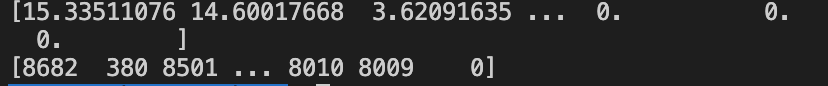
例如我们来看看其中一项结果，代码如下：

print(result[8456])print(result_indices[8456])

结果如下所示：

实际情况中，我们会根据经验对LLR分数进行一些限制，因此将不重要的指标会进行删除。

minLLR = 5indicators = result[:, :50]indicators[indicators < minLLR] = 0.0indicators_indices = result_indices[:, :50]max_indicator_indices = (indicators==0).argmax(axis=1)max = max_indicator_indices.max()indicators = indicators[:, :max+1]indicators_indices = indicators_indices[:, :max+1]

训练出结果后，我们可以将其放入到ElasticSearch中进行实时检索。使用到的Python依赖库如下：

import requestsimport json

这里使用ElasticSearch的批量更新API，创建一个新的索引，实现代码如下：

actions = []for i in range(indicators.shape[0]):    length = indicators[i].nonzero()[0].shape[0]    real_indicators = items[indicators_indices[i, :length]].astype("int").tolist()    id = items[i]        action = { "index" : { "_index" : "items2", "_id" : str(id) } }        data = {        "id": int(id),        "indicators": real_indicators    }        actions.append(json.dumps(action))    actions.append(json.dumps(data))        if len(actions) == 200:        actions_string = "\n".join(actions) + "\n"        actions = []                url = "http://127.0.0.1:9200/_bulk/"        headers = {            "Content-Type" : "application/x-ndjson"        }        requests.post(url, headers=headers, data=actions_string)if len(actions) > 0:    actions_string = "\n".join(actions) + "\n"    actions = []    url = "http://127.0.0.1:9200/_bulk/"    headers = {        "Content-Type" : "application/x-ndjson"    }    requests.post(url, headers=headers, data=actions_string)

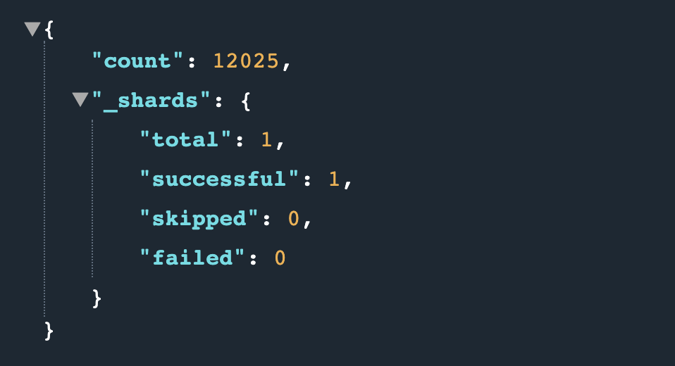
在浏览器中访问地址：

http://127.0.0.1:9200/items2/_count

结果如下所示：

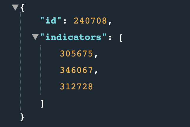
接下来，我们可以尝试将访问地址切换为：

http://127.0.0.1:9200/items2/240708

结果如下所示：

04 总结

构建一个面向生产环境的推荐系统并不困难，目前现有的技术组件可以满足我们构建这样一个生产环境的推荐系统。比如Hadoop、Hive、HBase、Kafka、ElasticSearch等这些成熟的开源组件来构建我们的生产环境推荐系统。本案例的完整代码如下所示：

import pandas as pdimport numpy as npfrom scipy.sparse import csr_matriximport requestsimport json
df = pd.read_csv('resource/events.csv')# print(df.shape)# print(df.head())# print(df.event.unique())trans = df[df['event'] == 'transaction']# print(trans.shape)# print(trans.head())
visitors = trans['visitorid'].unique()items = trans['itemid'].unique()# print(visitors.shape)# print(items.shape)
trans2 = trans.groupby(['visitorid']).head(50)# print(trans2.shape)
trans2['visitors'] = trans2['visitorid'].apply(lambda x : np.argwhere(visitors == x)[0][0])trans2['items'] = trans2['itemid'].apply(lambda x : np.argwhere(items == x)[0][0])
# print(trans2)occurences = csr_matrix((visitors.shape[0], items.shape[0]), dtype='int8')def set_occurences(visitor, item):    occurences[visitor, item] += 1trans2.apply(lambda row: set_occurences(row['visitors'], row['items']), axis=1)# print(occurences)
cooc = occurences.transpose().dot(occurences)cooc.setdiag(0)# print(cooc)
def xLogX(x):    return x * np.log(x) if x != 0 else 0.0def entropy(x1, x2=0, x3=0, x4=0):    return xLogX(x1 + x2 + x3 + x4) - xLogX(x1) - xLogX(x2) - xLogX(x3) - xLogX(x4)def LLR(k11, k12, k21, k22):    rowEntropy = entropy(k11 + k12, k21 + k22)    columnEntropy = entropy(k11 + k21, k12 + k22)    matrixEntropy = entropy(k11, k12, k21, k22)    if rowEntropy + columnEntropy < matrixEntropy:        return 0.0    return 2.0 * (rowEntropy + columnEntropy - matrixEntropy)def rootLLR(k11, k12, k21, k22):    llr = LLR(k11, k12, k21, k22)    sqrt = np.sqrt(llr)    if k11 * 1.0 / (k11 + k12) < k21 * 1.0 / (k21 + k22):        sqrt = -sqrt    return sqrt
row_sum = np.sum(cooc, axis=0).A.flatten()column_sum = np.sum(cooc, axis=1).A.flatten()total = np.sum(row_sum, axis=0)pp_score = csr_matrix((cooc.shape[0], cooc.shape[1]), dtype='double')cx = cooc.tocoo()for i,j,v in zip(cx.row, cx.col, cx.data):    if v != 0:        k11 = v        k12 = row_sum[i] - k11        k21 = column_sum[j] - k11        k22 = total - k11 - k12 - k21        pp_score[i,j] = rootLLR(k11, k12, k21, k22)    result = np.flip(np.sort(pp_score.A, axis=1), axis=1)result_indices = np.flip(np.argsort(pp_score.A, axis=1), axis=1)print(result.shape)
print(result[8456])print(result_indices[8456])
minLLR = 5indicators = result[:, :50]indicators[indicators < minLLR] = 0.0indicators_indices = result_indices[:, :50]max_indicator_indices = (indicators==0).argmax(axis=1)max = max_indicator_indices.max()indicators = indicators[:, :max+1]indicators_indices = indicators_indices[:, :max+1]
actions = []for i in range(indicators.shape[0]):    length = indicators[i].nonzero()[0].shape[0]    real_indicators = items[indicators_indices[i, :length]].astype("int").tolist()    id = items[i]        action = { "index" : { "_index" : "items2", "_id" : str(id) } }        data = {        "id": int(id),        "indicators": real_indicators    }        actions.append(json.dumps(action))    actions.append(json.dumps(data))        if len(actions) == 200:        actions_string = "\n".join(actions) + "\n"        actions = []                url = "http://127.0.0.1:9200/_bulk/"        headers = {            "Content-Type" : "application/x-ndjson"        }        requests.post(url, headers=headers, data=actions_string)if len(actions) > 0:    actions_string = "\n".join(actions) + "\n"    actions = []    url = "http://127.0.0.1:9200/_bulk/"    headers = {        "Content-Type" : "application/x-ndjson"    }    requests.post(url, headers=headers, data=actions_string)